As the name implies, linear regression solves a regression problem. The goal is to build a system that can take an input vector \(x \in \mathbb{R}^n\) and predict the value of a scalar \(y \in \mathbb{R}\).

The output of linear regression is a linear function of the input. Hence, the output function can be defined as:

$$ y = w^T x\,. $$

where \(w\) is a vector of paramters that must be the same size of \(x\) \(\in \mathbb{R}^n\).

If a feature’s weight \(w_i\) is large in magnitude, then it has a large effect on the prediction. If a feature’s weight is zero, it has no effect on the prediction.

To make a machine learning algorithm, we need to design an algorithm that will improve the weights \(w\) in a way that reduces MSE. One intuitive way of doing this is just to minimize the mean squared error on the training set, and, to minimize the MSE during training that we can simply solve for where the gradient is \(0\):

$$ \text{MSE} = \frac{1}{m} ||\hat{y} - y ||_2^2\,, $$ $$ \triangledown_w\; \frac{1}{m} ||\hat{y} - y ||_2^2 = 0\,. $$

Note that the \(\hat{y}\) with the hat is our prediction, and the \(y\) is the test label.

We can calculate this gradient with the Linear Least Squares method which we previously did in the following blog post: Solving the Linear Least Squares problem with the Gradient.

Also, note that with the multi-variate regression we have the following prediction formula:

$$ \hat{y} = Xw\, $$

because our input will now be a matrix.

In order to solve for the gradient we need to substitute for our output function and expand our \(L^2-\)norm, that we can express as the dot product with the transpose. And then differentiate the resulting expression by expressing the terms as sums, this way we can apply normal scalar differentiation.

$$ \triangledown_w\; \frac{1}{m} ||\hat{y} - y ||_2^2 = 0\,, $$ $$ \frac{1}{m} \triangledown_w\;||Xw - y ||_2^2 = 0\,, $$ $$ \frac{1}{m} \triangledown_w\;(Xw - y)^T(Xw - y) = 0\,, $$ $$ \frac{1}{m} \triangledown_w\;(w^TX^T - y^T)(Xw - y) = 0\,, $$ $$ \frac{1}{m} \triangledown_w\;(w^TX^TXw - w^TX^Ty - y^TXw + y^Ty) = 0\,, $$ $$ \frac{1}{m} \triangledown_w\;2XX^Tw - 2X^Ty = 0\, $$

Now solving for \(w\) we have: $$ 2XX^Tw = 2X^Ty\,, $$ $$ XX^Tw = X^Ty\,, $$ $$ w = (XX^T)^{-1}X^Ty\,. $$

Practical Example on Linear Uni-variate Regression

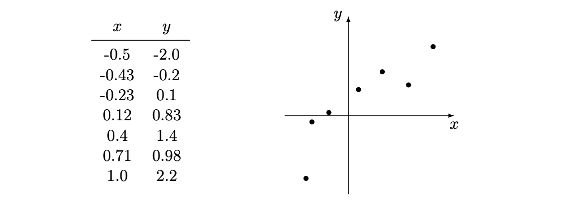
We have the following data, where \(x\) is the dependent variable and \(y\) the independent. We would like to predict \(y\).

$$ w=(XX^T)^{-1}X^Ty\,, $$

Note that for \((XX^T)\) to have an inverse, we need to avoid singular matrices where the determinant is zero. Therefore, we add a mock feature that won't change our results, of all ones.

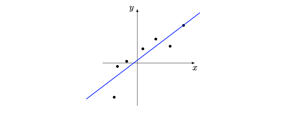
$$ XX^T = \begin{pmatrix} 7 & 1.07\\ 1.07 & 2.16\\ \end{pmatrix}\,, $$ $$ (XX^T)^{-1} = \begin{pmatrix} 0.15 & -0.7\\ -0.07 & 0.49\\ \end{pmatrix}\,, $$ $$ X^Ty = \begin{pmatrix} 3.31\\ 4.61\\ \end{pmatrix}\,, $$ $$ w = (XX^T)^{-1}X^Ty = \begin{pmatrix} 0.15 & 2.05\\ \end{pmatrix}\,. $$

Now we have our weights we can do any prediction we want given an \(x\) value:

$$ y_{test} = X_{test}\;w\,. $$

Giving us the corresponding line:

Code

References

• Probabilistic Machine Learning: An Introduction, Kevin P. Murphy (2022)
• MLPR 2022: Regression and Gradients (Notes), University of Edinburgh (2022)